1 Abstract
We have profiled the various pipetasks in the DRP pipeline and have characterized the memory and CPU time usage of those tasks for processing DESC DC2 data. We have also studied the efficiency of running on Rome and Milan processors at various levels of node occupancy. This information is used to estimate the node hours required to do the first year of DRP processing of the Rubin WFD survey.
2 Motivation and Background
This study was originally motivated by the need for the Dark Energy Science Collaboration (DESC) to understand its computing resource needs for systematics assessments that require pixel-level reprocessing of the first year (Y1) of Rubin data. In practice, these assessments would involve the reprocessing of several smaller data sets, using alternative algorithms and/or data selections, or could include simulated images. Therefore, as rough guide to the needed resources, DESC settled on the goal of reprocessing 10% of Y1 data 10 times as the target workload for this study. For simplicity, we’ve recast this as doing a full DRP processing of the Y1 Wide Fast Deep (WFD) Rubin observations. The WFD survey comprises ~80% of the Y1 data, and it provides a relatively homogeneous data set that’s relevant for DESC’s needs and which makes the resource estimation straight forward.
3 Inputs to Estimating the Y1 WFD DRP Processing
The basic input to this study is the cadence of observations during Y1. We have used version v2.0 of the 10 year baseline cadence that is available from the UW server as baseline_v2.0_10yrs.db. In Figure 1, we plot the pointing centers for Y1 for the 7 different “proposalIds” in the observations table in the baseline cadence file. The legend shows the number of visits for each proposalId: the blue points correspond to pointings that cover the Galactic plane and North Ecliptic Spur, the orange points correspond to the WFD survey, and the remaining 5 proposalIds correspond to Deep Drilling Fields. In Table 1, we show the number of visits per band in the Y1 WFD observations.
Figure 1: Pointing directions of Y1 visits from baseline cadence v2.0.
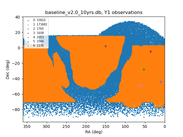
Table 1: Number of visits per band for Y1 WFD
| band | # visits |
|---|---|
| u | 11068 |
| g | 14628 |
| r | 35258 |
| i | 39851 |
| z | 32211 |
| y | 40666 |
4 Estimation Procedure
There are a lot of individual pipetasks in the nominal DRP pipeline, and only a subset of them require a substantial amount of computing resources, so for this study, we’ve only considered those pipetasks in our estimates. By counting the number of instances of each kind of pipetask involved in processing the full Y1 data set, we can estimate the number of “node-days” required to process those data assuming that the number of concurrent jobs that we can run on a node is limited by the node’s memory and the number of available cores.
Given a particular observing cadence, we can extract some key numbers that will give us precise numbers of instances for the visit-level pipetasks, and we can make reasonably close estimates, i.e., within factors of 1.4 or less, for the remaining ones. For example, for the Y1 WFD survey in the baseline v2.0 cadence, there are 173,682 visits, which when multiplied by the number of science CCDs in the LSSTCam focal plane, 189, yields ~33 million instances of each of the single frame processing pipetasks. For the pipetasks that operate on coadds, the number of instances depends on the sky map used. For the DC2 sky map, there are a total of 18,938 tracts and 49 patches per tract. Estimating the WFD survey to cover 18k square degrees, this yields ~460,000 patches and ~2.5 million coadds, using 6 LSST bands per patch.
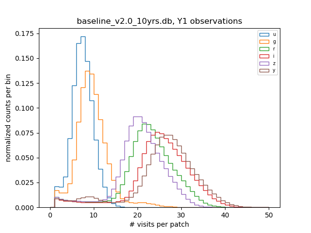
It’s somewhat more difficult to estimate the numbers of visits per patch per band. As we’ll see in the next section, these numbers are relevant for the resource scaling of many of the coadd-level tasks. To get more precise estimates of these numbers, we simulate the baseline cadence pointings and find the number of overlaps of the focal plane projected onto the DC2 sky map with each patch. Here we model the extent of the focal plane as a circle on the sky with radius ~2 degrees. In Figure 2, we show the distributions of number of visits per patch for each of the six LSST bands that were obtained by this procedure for the Y1 WFD observations.
Figure 2: Number of visits per patch for Y1 WFD baseline 2.0 observations using the DC2 sky map
5 Profiling the Individual Pipetasks
Note that all results presented in sections 5-7 used lsst_distrib weeklies w_2021_21, w_2021_22, and w_2021_33.
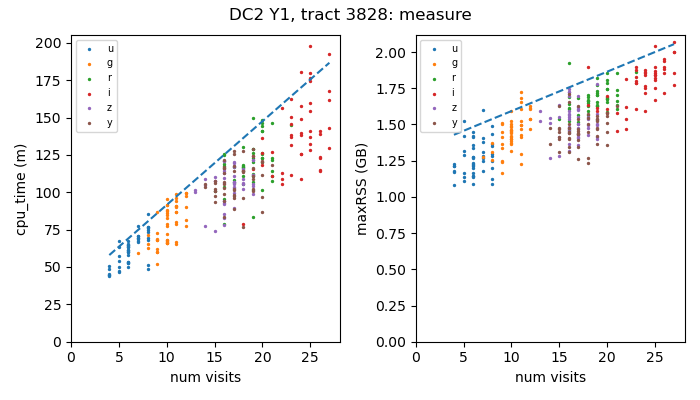
In order to determine the resource requirements for each pipetask instance, we’ve profiled the various pipetasks by running the static science part of the DRP pipeline on tract 3828 of the Y1 DC2 data and harvested the metadata files that are produced. These files contain per-process information such as the total CPU time used and the maximum memory that was required, i.e., the maximum resident set size (maxRSS). Pipetasks that operate on visit-level data have relatively narrow-ranges of CPU time usage and maxRSS values. For example, as shown in Figure 3, running on Cori-Haswell nodes at NERSC, the calibrate pipetask typically needs ~0.5-1.5 CPU minutes and ~0.79 GB of maxRSS memory. By contrast, for the pipetasks that analyze the coadded images, both the CPU time and maxRSS values scale with the number of visits included in the coadd (See Figure 4). For estimating resource needs for visit-level pipetasks, we take the 95-th percentile value of the CPU time or maxRSS distributions (dotted vertical lines in Figure 3). For the coadd-level pipetasks, we model the resource needs using a linear fit to the upper envelope of points in the plots of either CPU time or maxRSS versus number of visits in the coadd. For those plots, the number of visits for a given patch is determined by averaging over the corresponding nImage FITS file, which contains the number of visit-level images contributing to each coadd pixel.
Figure 3: CPU time and maxRSS distributions for the calibrate pipetask
running on Cori-Haswell nodes at NERSC
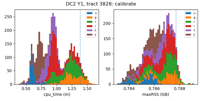
Figure 4: CPU time and maxRSS versus the mean number of visits in the coadd
for the measure pipetask running on Cori-Haswell nodes at NERSC
6 Processing Time Results
Combining the per-instance resource estimates for each pipetask with the per-instance information for each pipetask that we gathered from our simulation of the pointings, we obtain the following table of per-instance resource requirements, derived from the actual distributions of pipetask instances as a function of number of visits. Here CPU hours is total number of CPU hours integrated over those distributions, and max(maxRSS) is the maximum of the distribution of maxRSS values. We can use this latter value to obtain a conservative constraint on the number of jobs can be run concurrently on a node that has a given amount of memory.
Table 2: Estimated CPU and memory requirements for key DRP pipetasks averaged over the Y1 WFD pointings
| pipetask | # instances (M) | CPU hours (M) | max(maxRSS) (GB) |
|---|---|---|---|
| isr | 32.8 | 0.64 | 2.59 |
| characterizeImage | 32.8 | 1.23 | 0.83 |
| calibrate | 32.8 | 0.76 | 0.79 |
| makeWarp | 48.5 | 2.83 | 3.20 |
| assembleCoadd | 2.7 | 0.44 | 1.48 |
| detection | 2.7 | 0.12 | 1.39 |
| measure | 2.7 | 6.12 | 2.79 |
| forcedPhotCoadd | 2.7 | 7.56 | 1.77 |
| deblend | 0.4 | 0.79 | 6.98 |
As noted, this profiling was done using Cori-Haswell nodes at NERSC. For running on platforms with different processors and memory configurations, we expect the overall processing time to scale with the execution speed of the tasks on those processors, subject to constraints imposed by the memory and the number of cores per node. Taking all that into account, Table 3 shows the overall processing time estimates for the three different systems that will be available at NERSC in late 2022. The CPU factor of 8 for Cori-KNL was determined empirically by running the DRP code on those nodes, while the CPU factor of 1 for Perlmutter is a conservative estimate that we made before the Perlmutter system was available at NERSC. As we’ll see below, for the instrument signature removal (ISR) pipetask, the execution time on a Perlmutter CPU is about a factor of ~2 smaller than the time to run on a Cori-Haswell CPU.
Table 3: Overall processing time estimates
| platform | CPU factor | cores per node | memory per node (GB) | node days (k) |
|---|---|---|---|---|
| Cori-KNL | 8 | 68 | 96 | 198 |
| Cori-Haswell | 1 | 32 | 128 | 28 |
| Perlmutter* | 1 | 128 | 512 | 7 |
In Table 3, we use the configuration of Perlmutter CPU nodes that are expected when the Perlmutter phase 2 installation at NERSC has completed. This configuration will be similar to the “rome” nodes at SLAC SDF, except that Perlmutter will use Milan processors, while SDF nodes use Rome processors.
7 Disk Storage Needs
In order to assess disk storage needs, we’ve computed the average file sizes for the different data set types, and in Table 4 we show the DRP data product data set types that would take up >50TB of disk space. Retaining all of these data products would require ~21 PB of disk space. Based on the compressed raw image file sizes for DC2, ~20 MB per file, the Y1 WFD raw data volume would be 0.66 PB, implying a factor of ~32 increase in data volume for the DRP outputs. Most of the data products produced by the DRP pipeline aren’t needed long term. The ones that DESC found useful for running its downstream validations and analyses are marked with Y in the Keep? column. Keeping those data sets yields 4.2 PB, which is about a factor ~6 increase in data volume.
Table 4: DRP data products with >50TB total disk usage
| task | dataset type | avg. file size (MB) | # instances (M) | Y1 totals (TB) | Keep? |
|---|---|---|---|---|---|
| isr | postISRCCD | 91.6 | 33.8 | 2870 | |
| characterizeImage | icExp | 103.0 | 33.8 | 3230 | |
| calibrate | calexp | 103.2 | 33.8 | 3230 | Y |
| calibrate | src | 5.4 | 33.8 | 170 | Y |
| makeWarp | deepCoadd_directWarp | 104.5 | 48.5 | 4830 | |
| makeWarp | deepCoadd_psfMatchedWarp | 100.7 | 48.5 | 4650 | |
| assembleCoadd | deepCoadd_nImage | 33.6 | 2.7 | 90 | Y |
| assembleCoadd | deepCoadd | 117.8 | 2.7 | 300 | |
| detection | deepCoadd_calexp | 117.9 | 2.7 | 300 | Y |
| deblend | deepCoadd_deblendedFlux | 126.5 | 0.4 | 50 | |
| measure | deepCoadd_meas | 166.6 | 2.7 | 430 | |
| forcedPhotCoadd | deepCoadd_forced_src | 164.8 | 2.7 | 420 | Y |
8 Throughput Scaling with Node Occupancy
The results in this section used lsst_distrib weeklies w_2021_42 for Perlmutter, w_2021_48 for Cori-KNL and Cori-Haswell, and w_2022_02 for SLAC-SDF.
The estimates above of the overall processing times assume that job throughput scales linearly with the number of concurrent processes, assuming that on any given node, there are fewer processes than the number of cores. However, contention for resources like memory bandwidth, cache space, or disk access can cause jobs to run more slowly as the number of concurrent processes increases. In addition, thermal power limitations can reduce the CPU clock speeds from their maximum values if the compute load on the node is very high.
In order to characterize the job throughput scaling as a function of node occupancy, we’ve run several thousand ISR pipetask jobs (as defined in the DRP pipeline) on DC2 data for different numbers of concurrent processes, up to the number of available cores. We’ve done this on the SDF-Rome nodes as well as on the Cori-KNL, Cori-Haswell, and Perlmutter phase 1 systems at NERSC. For all four systems, we see similar behavior: For small numbers of concurrent processes (e.g., fewer than 32 on SDF), the throughput scales roughly linearly, and plateaus at higher loads.
So that we can maintain a constant load on those systems, we used the ISR task since its resource usage is largely independent of the input data; and rather than relying on a workflow management system like Parsl (which may have some overhead that we can’t control) to schedule the jobs, we reserved exclusive nodes in the slurm queues at SDF and at NERSC, and used the python subprocess and multiprocessing modules in a special purpose script to control the number of concurrent processes very precisely.
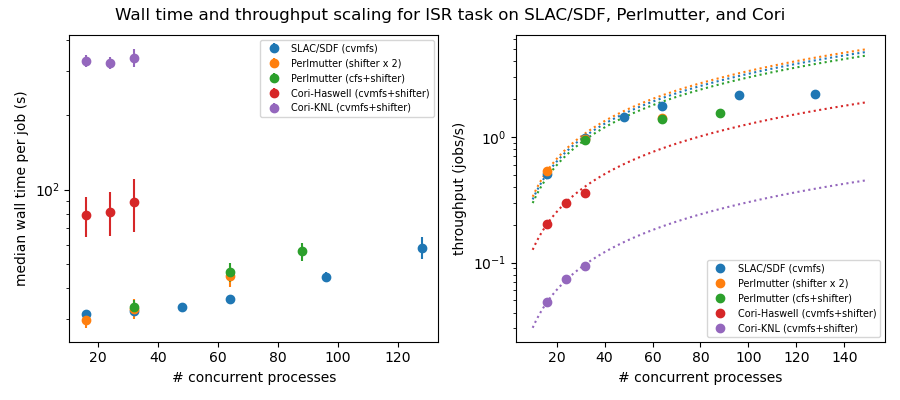
Figure 5 shows the results of these tests. The plot on the left shows the mean wall time for the ensemble of ISR jobs as a function of the number of concurrent processes. For # concurrent processes > 48, we see significant departures from constant wall time on the SDF and Perlmutter systems (the Cori systems have either too few cores or too little memory to support this many ISR jobs). The plot on the right shows the same data except with the throughput (jobs/s) plotted versus # concurrent processes. The dotted curves show the expected linear scaling, extrapolating from the 16-process value. At the worst case, for 128 concurrent processes on SDF-Rome, the relative degradation in throughput is a factor ~2 relative to linear scaling.
Figure 5: Throughput scaling for the ISR task on SLAC/SDF, Perlmutter, and Cori
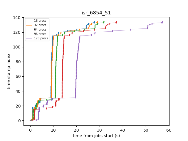
Following a suggestion from K-T, we enabled debug-level logging in order to determine what’s happening during the job when the slowdowns are occurring. Apart from the time stamps, the log entries are the same for a given ISR instance, so we can easily match up entries and see directly how the wall time for specific operations scale with the number of concurrent processes. Figure 6 shows an example plot of time stamp index versus wall time from the start of a particular ISR job. We’ve filtered the time stamps to include just operations that involve either datastore I/O-related activities, indicated by stars in the plot, or compute intensive tasks, such as computing pixel statistics, applying crosstalk correction, or deconvolving the Brighter-Fatter kernel, which are all indicated by points. The fact that the datastore I/O parts of the time histories cross indicates that disk activity on the cluster from other nodes is probably affecting those operations.
Figure 6: Time stamps vs job wall time for an ISR task instance running with different levels of node occupancy.
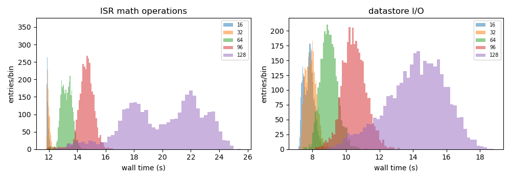
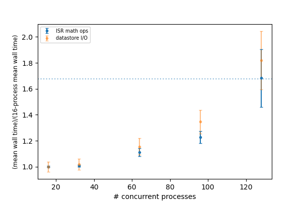
In Figure 7, we plot the distributions of job wall times for the compute-intensive operations (left) and for the datastore operations (right). For the compute-intensive slowdowns, Adrian Pope suggested that clock speed scaling of the CPU may be occurring. At very high loads, the CPUs will approach the Thermal Design Power (TDP) limit where the average clock speeds are at the ~base frequency of the CPU. At low loads, the cores can run closer to the maximum boost speed, so the fact that the compute-intensive wall time distributions are sharply peaked at 12 s for 16 and 32 concurrent processes strongly suggests that the cores are running at the maximum boost speed. For the SDF-Rome CPUs, the maximum boost speed is 3.35 GHz, while the base frequency is 2.0 GHz. So if the jobs in the 128-process runs are suffering from TDP frequency scaling, their average wall times should be ~3.35/2.0 longer than the 16-process runs, or ~20 s.
Figure 7: Distributions of wall times for compute- and datastore-intensive operations.
To illustrate this more explicitly, in Figure 8, we plot the mean wall times for compute- and datastore-intensive operations versus # concurrent process, scaled to the 16-process values. The wall time scalings for compute and datastore operations are clearly different, as we would expect. The horizontal dotted line is the ratio of the maximum boost frequency to the base frequency for SDF-Rome CPUs, and it suggestively passes through the 128-process point. Notably, monitoring of /proc/cpuinfo while running on an SDF-Rome node seems to indicate that the nodes are locked at their CPU base frequencies of 2 GHz. However, using the perf tool to profile the ISR pipetasks shows that several effects, includng TDP scaling, are affecting the overall throughput as a function of the number of concurrent processes.
Figure 8: Mean wall time for compute- and datastore-intensive operations versus #concurrent processes.
8.1 Using perf to profile the DRP pipetasks
In order to obtain additional information on the state of the CPU while the pipetask jobs are executing, we used the perf tool to gather statistics from various performance counters for each job. Prepending the perf stat -d command to each pipetask job command line yields output similar to that shown in Figure 9.
Figure 9: perf stat -d output for a job from a 16 concurrent process run.
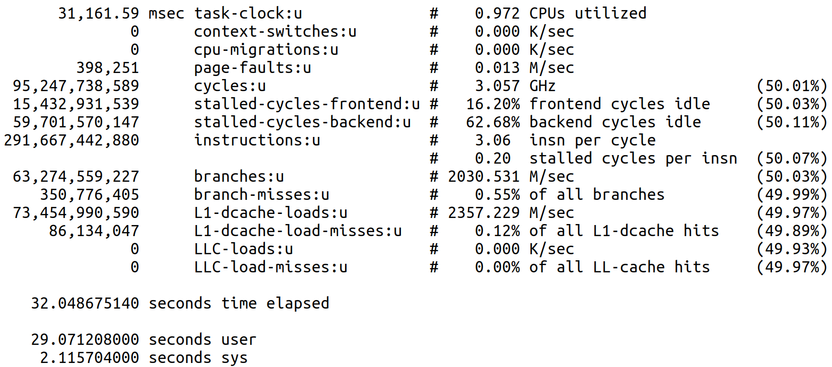
There are several quantities of interest in this output for understanding the performance scaling of these jobs. Since the ISR task executes basically the same set of operations regardless of the input data, the number of instructions for all the jobs is essentially constant, i.e., ~2.9e11 instructions. The cycles required to execute these instructions can vary if there is contention for resources, e.g., contention for L3 cache among the CPUs sharing that memory will result in LLC-load-misses, which, in turn, will increase the number of cycles used. Another important quantity is the task-clock time, which, divided into cycles, yields the CPU frequency or clock speed. In the above example, the CPU frequency is 3.057 GHz, higher than the 2.0 GHz base frequency, indicating that this CPU is not running at its TDP limit. Finally, the time elapsed, user, and sys times can be used to infer the time that the process spends outside of user or kernel code, i.e., the time spent doing disk I/O or being blocked by other processes using the CPU (if hyperthreading). As long as #concurrent jobs is less than the number of available cores, the difference time elapsed - (user + sys) should provide a measure of the time spent doing disk I/O, with larger values of that difference indicating contention for disk access.
For 128 concurrent processes, we see quite different perf stat -d output for the same ISR job (Figure 10):
Figure 10: perf stat -d output for a job from a 128 concurrent process run.
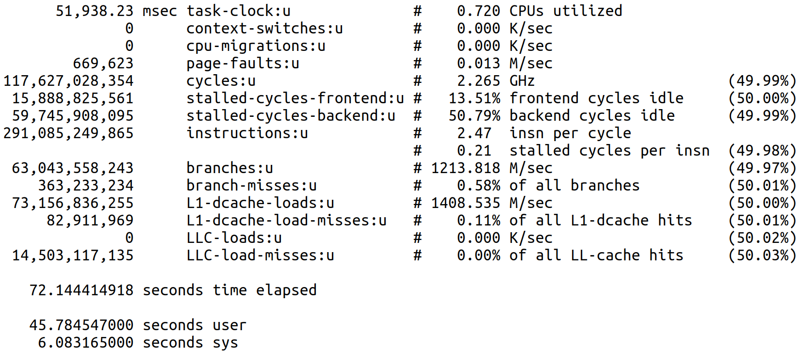
The number of LLC-load-misses is significantly different from zero and corresponds roughly to the increase in cycles relative to the 16-process case. However, even though cycles increases, the task-clock value increases even more, resulting in a clock speed of 2.265 GHz, clearly indicating that TDP scaling is occurring. Lastly, the difference time elapsed - (user + sys) also increases, consistent with higher disk I/O contention for the larger number of concurrent processes.
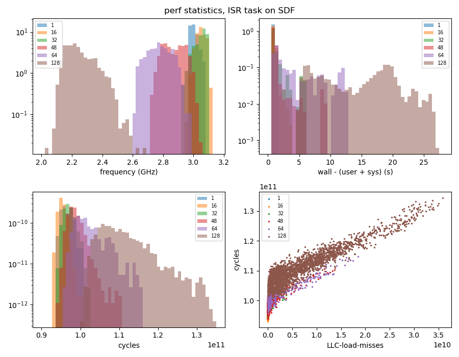
In Figure 11, we show the distributions of these three resource contention metrics: CPU frequency (upper left), wall - (user + sys) time (upper right), and #cycles (lower left), for runs with different numbers of concurrent processes, showing clear scaling with node occupancy. In the lower right panel, we also plot cycles vs LLC-load-misses to show the strong correlation between these two quantities.
Figure 11: Distributions of resource contention metrics for different numbers of concurrent processes.